The Life, Death, and Zombification of the Phillips Curve

The Rise and Fall of One of the Most Important Concepts in Macroeconomics

The views expressed in this blog are entirely my own and do not necessarily represent the views of the Bureau of Labor Statistics or the United States Government.

Thanks for reading. If you haven’t subscribed, please click the button below:

Otherwise, liking or sharing is the best way to support my work. Thank you!

In 1958 economist Alban William Phillips published “The Relation Between Unemployment and the Rate of Change of Money Wage Rates in the United Kingdom, 1861–1957” in which he demonstrated a correlation between the growth of nominal wages and unemployment. When unemployment was low nominal wages tended to grow faster, and when unemployment was high nominal wages tended to grow slower.

Over the ensuing decades the Phillips curve evolved into a codified relationship between inflation (not wage growth) and unemployment. In the traditional story, stimulating demand would decrease unemployment at the cost of increased inflation, and decreasing demand would boost unemployment while decreasing inflation. There was an assumed stable tradeoff between unemployment and inflation: any effort to reduce unemployment required an increase in inflation and any effort to lower inflation required an increase in unemployment.

The experience of the 1970s stagflation and the influence of the Chicago school of economics radically transformed the Phillips curve. Monetarist economists posited that long run inflation was driven by growth in the money supply, and therefore high unemployment could coexist with high inflation. Expectations were critical to this story: when consumers and producers expected large growth in the money supply and commensurately high inflation they would make wage, price, and purchase decisions based on these expectations. Expected inflation would move through these channels to cause equally high realized inflation.

The monetarist revolution was unable to kill the Phillips curve, however, and the idea persisted in a zombified state under the “expectations augmented Phillips curve.” There was no long run relationship between unemployment and inflation, as long term inflation was a monetary phenomenon. In the short run, however, the Phillips curve persisted—it was assumed that the central bank still faced an immediate tradeoff between unemployment and inflation.

In the decades after the 1970s inflation was defeated, even the short-run Phillips curve relationship began breaking down. The Federal Reserve became successful in containing inflation in what was dubbed “The Great Moderation”—and coincidentally the Phillips curve supposedly “flattened” as the relationship between inflation and unemployment weakened.

Lots of ink was spilled in the ensuing years regarding the flattening of the Phillips curve relationship and its possible causes: globalization, monetary policy, stable inflation expectations, changing labor markets, and more. In recent years a new swathe of evidence has supported another explanation: that there simply is no consistent law-like relationship between inflation and unemployment.

Death

As for the Phillips curve…most arguments today center around whether it’s dead or just gravely ill. Either way, the relationship between unemployment and inflation has become very difficult to spot.

Federal Reserve Bank of San Francisco President Dr. Mary Daly

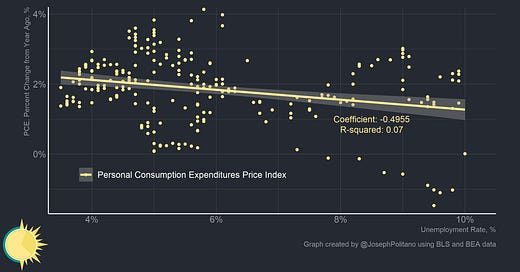
Over the last 20 years, the Phillips curve relationship has nearly completely broken down in the United States. The chart above plots the monthly unemployment rate against the rate of inflation from the Personal Consumption Expenditures Price Index (PCEPI) from January 2000 to January 2020. The relationship itself is astoundingly flat—a 10% unemployment rate represents approximately 1.6% inflation on the fitted linear regression model while 4% unemployment represents 2% inflation. The coefficient of determination (R-squared) is also incredibly low, indicating that a low proportion of variation in inflation is predictable by unemployment.

It should be noted that this is among the most generous measurements of the Phillips curve relationship, and yet no strong correlation is discernable. The relationship is statistically significant, but this is before accounting for correlated errors (the tendency of unaccounted for factors to influence the relationship in nonrandom ways) or autocorrelation (the relationship between data and its lagged values). In short, this just shows the correlation across time, it does not robustly demonstrate that there is a relationship. Even with this generous measurement, the traditional Phillips curve comes up extremely flat.

This is also true outside the United States, as demonstrated in the chart above. The Phillips curves for Japan, Canada, and the United Kingdom are all relatively flat. The UK’s Phillips curve is actually completely inverted, meaning higher unemployment is correlated with higher inflation!

This breakdown in the observed Phillips curve relationship is usually blamed on the stability of monetary policy and the endogeneity of monetary policy to both inflation and unemployment. In short, monetary policy has stabilized inflation expectations during the global “Great Moderation” and works to counteract the jumps in unemployment caused by recessions. If a central bank is effectively targeting inflation, then inflation will have no relationship with unemployment.

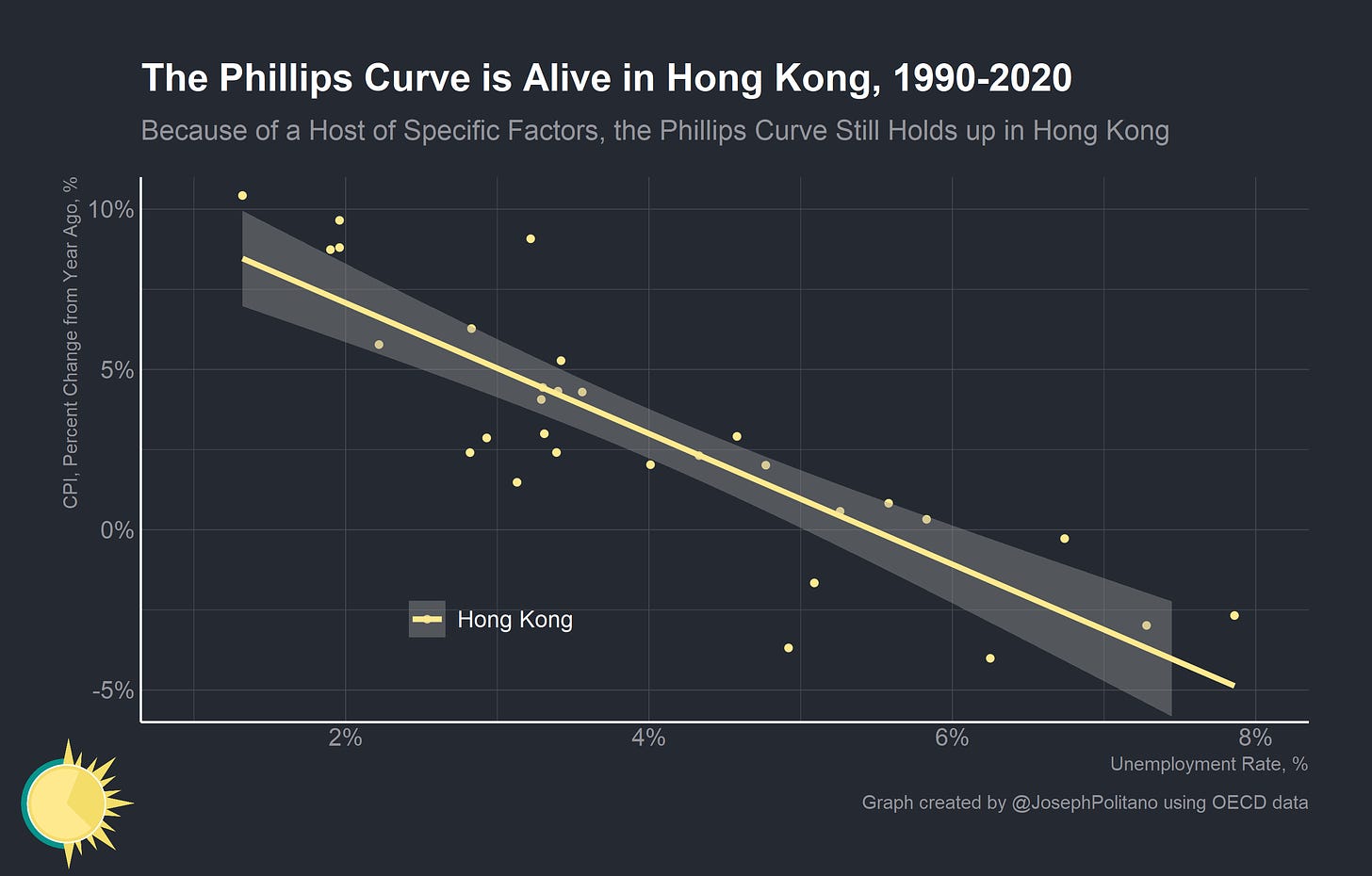
It therefore stands to reason that if monetary policy is exogenous (as in, is not targeting either unemployment or inflation) the Phillips curve relationship will resurface. Indeed, many people point to Hong Kong as an example of a strong Phillips curve caused by exogenous monetary policy. Hong Kong Dollars are pegged to the US Dollar, so the Federal Reserve effectively sets monetary policy in Hong Kong. The result is stable inflation expectations (as the Federal Reserve keeps US inflation at a constant 2%) alongside a large variance in inflation and unemployment (as the Federal Reserve ignores conditions in Hong Kong when setting monetary policy). The combination of stable inflation expectations, demand-driven economic growth, exogenous monetary policy, laissez-faire labor market, and large variance in unemployment and inflation generates a stable Phillips curve in Hong Kong.

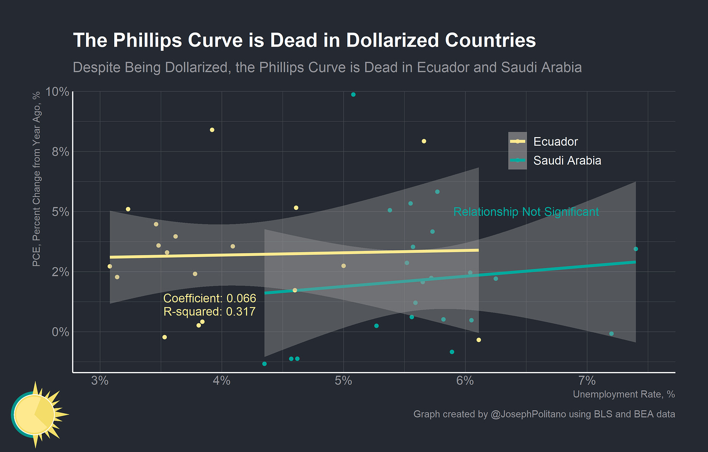
However, even other Dollarized economies do not show the same strong Phillips curve relationship! Ecuador adopted the US dollar as its currency in 2000 following an inflation crisis and Saudi Arabia pegged its currency to the dollar in 1986. Despite both countries having the same stable inflation expectations, exogenous monetary policy, and variance in unemployment and inflation, neither exhibits a Phillips curve relationship.

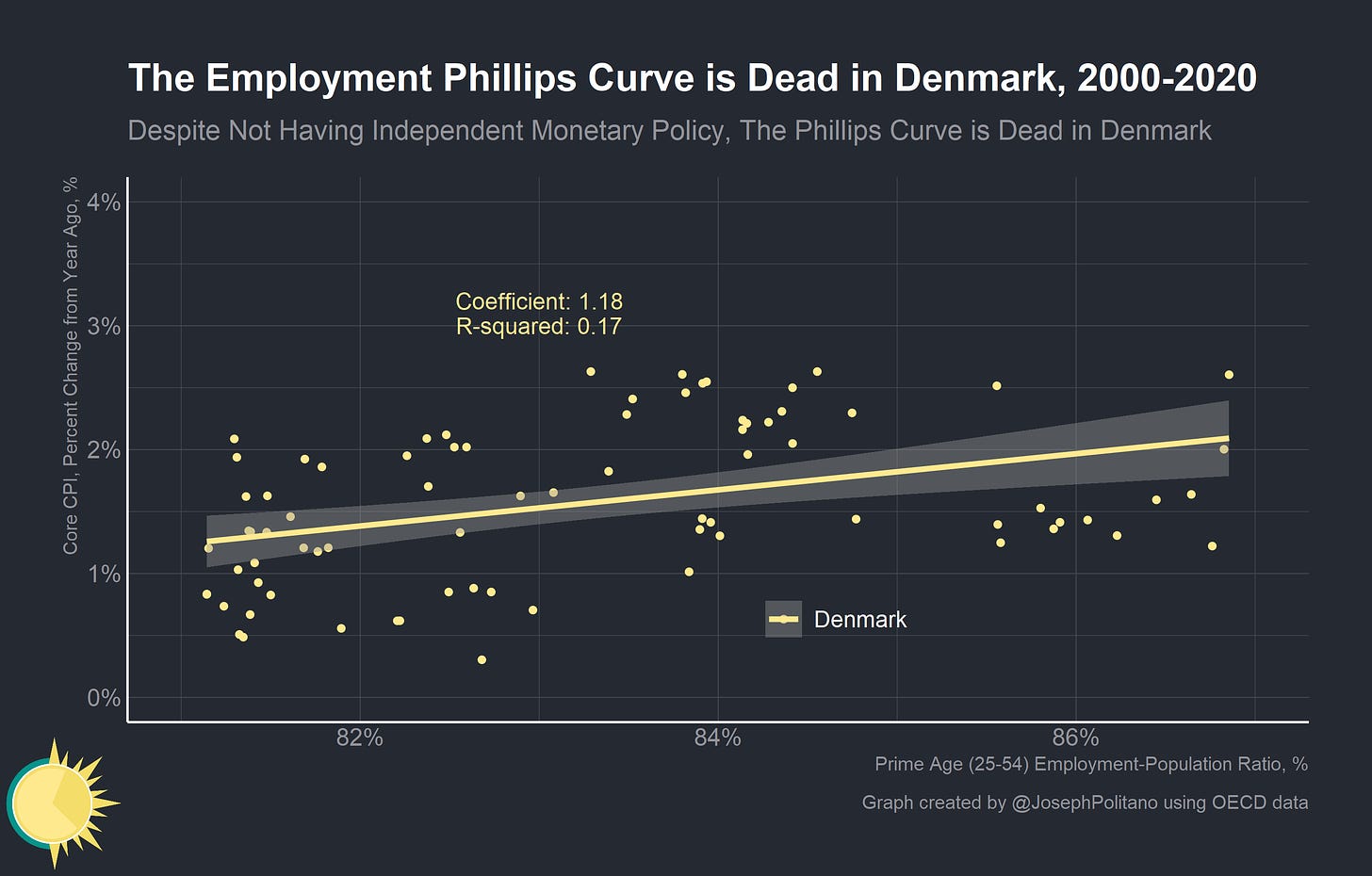
Denmark’s currency is pegged to the Euro, meaning they also lack independent monetary policy (although it would be a stretch to say that monetary policy is perfectly exogenous in Denmark, as the macroeconomic factors influencing Denmark are also likely influencing the rest of the Eurozone). They too exhibit a relatively flat Phillips curve relationship.

Therefore even exogenous monetary policy does not guarantee a Phillips curve relationship! Of course, exogenous monetary policy does likely increase the probability that a Phillips curve relationships is observable. This is because variance in the relative looseness or tightness of monetary policy will tend to drive both unemployment and inflation when policy is exogenous. Phillips’ own work was done primarily on periods in UK history when the gold standard made monetary policy exogenous to inflation and unemployment.

However, it does demonstrate how poor a framework the Phillips curve is given that modern central banks work to manage inflation and unemployment as part of their mandates. If the Phillips curve barely holds when monetary policy is exogenous, it is no wonder that it rarely holds when monetary policy is endogenous! Despite this, policymakers have incorporated concepts like the “non-accelerating inflation rate of unemployment” (NAIRU), which states that there is a certain unemployment rate that keeps inflation stable, into monetary and fiscal policymaking. These concepts have led to the Federal Reserve and other institutions constantly underestimating how low unemployment could go and pre-emptively tightening policy before the economy reached full employment.

Zombification

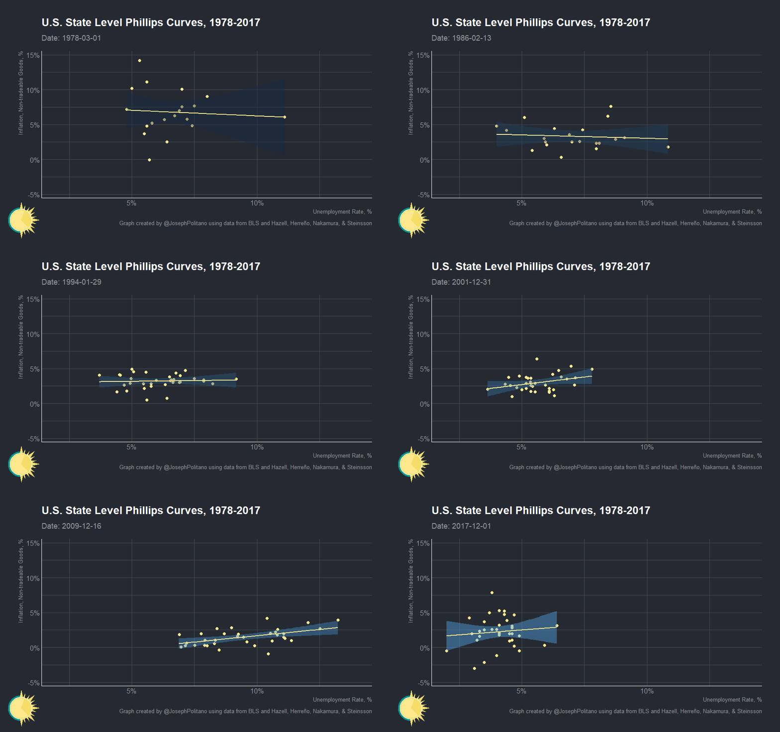
Our cross-sectional estimates indicate that the slope of the Phillips curve is small and was small even during the 1980s. They imply that only a modest fraction of the large changes in inflation in the early 1980s can be accounted for by the direct effect of increasing unemployment working through the slope of the Phillips curve.

The Slope of the Phillips Curve: Evidence from U.S. States

Hazell, Herreño, Nakamura, Steinsson (2021)

Recent efforts to robustly examine the Phillips curve have cast doubt on the idea that the relationship ever “flattened” as the conventional wisdom holds. More specifically, they demonstrate that the relationship was always “flat” and that the observations of seemingly strong Phillips curves were mostly artifacts of limited data analysis.

In their recent working paper “The Slope of the Phillips Curve: Evidence from U.S. States” Jonathon Hazell, Juan Herreño, Emi Nakamura, and Jón Steinsson constructed state-level price indexes of non-tradeable goods and used them to measure the slope of the Phillips curve. Their results showed that the Phillips curve was always relatively flat and that the bulk of changes in inflation cannot be explained through changes in unemployment.

The paper “Prospects for Inflation in a High Pressure Economy: is the Phillips Curve Dead or is it Just Hibernating?” by Peter Hooper, Frederic Mishkin, and Amir Sufi found marginally higher estimates using state level wage data and metropolitan statistical area (MSA) core inflation data. However, they did not construct equivalent non-tradeable price indexes like Hazell, Herreño, Nakamura, and Steinsson and did not perform equivalent statistical analyses.

It’s worth reflecting on the high level of specification required to construct a robust Phillips curve. Tradeable goods, which are a large and growing part of the increasingly globalized US economy, had to be completely excluded and national-level examination proved nearly impossible. Even still, the Phillips curve relationship is not particularly stable over short periods of time—the only time periods in which it is supposedly effective. It is unwise to attempt to target national level aggregate inflation using national level aggregate unemployment when even the state level non-tradeable Phillips curve relationship is weak.

At a broad level, unemployment is simply an extremely poor proxy for labor utilization, which itself is a poor proxy for total capacity utilization. Measurements of unemployment exclude discouraged workers (those who left the labor force entirely because they were unable to secure a job). They do not account for underemployment, where employed workers are forced to work part-time for economic reasons or cannot land a job that matches their skill specializations. Finally, it does not account for real wage growth at all—a weak labor market can sustain high employment levels alongside low wage growth. Finally, while labor utilization is the most important measure of capacity utilization by a wide margin, it is by no means the only measure of capacity utilization. Structural issues like inequality, regulatory capture, specific supply shocks, corporate mismanagement, or state excess can cause the economy to hit full capacity utilization without full labor utilization.

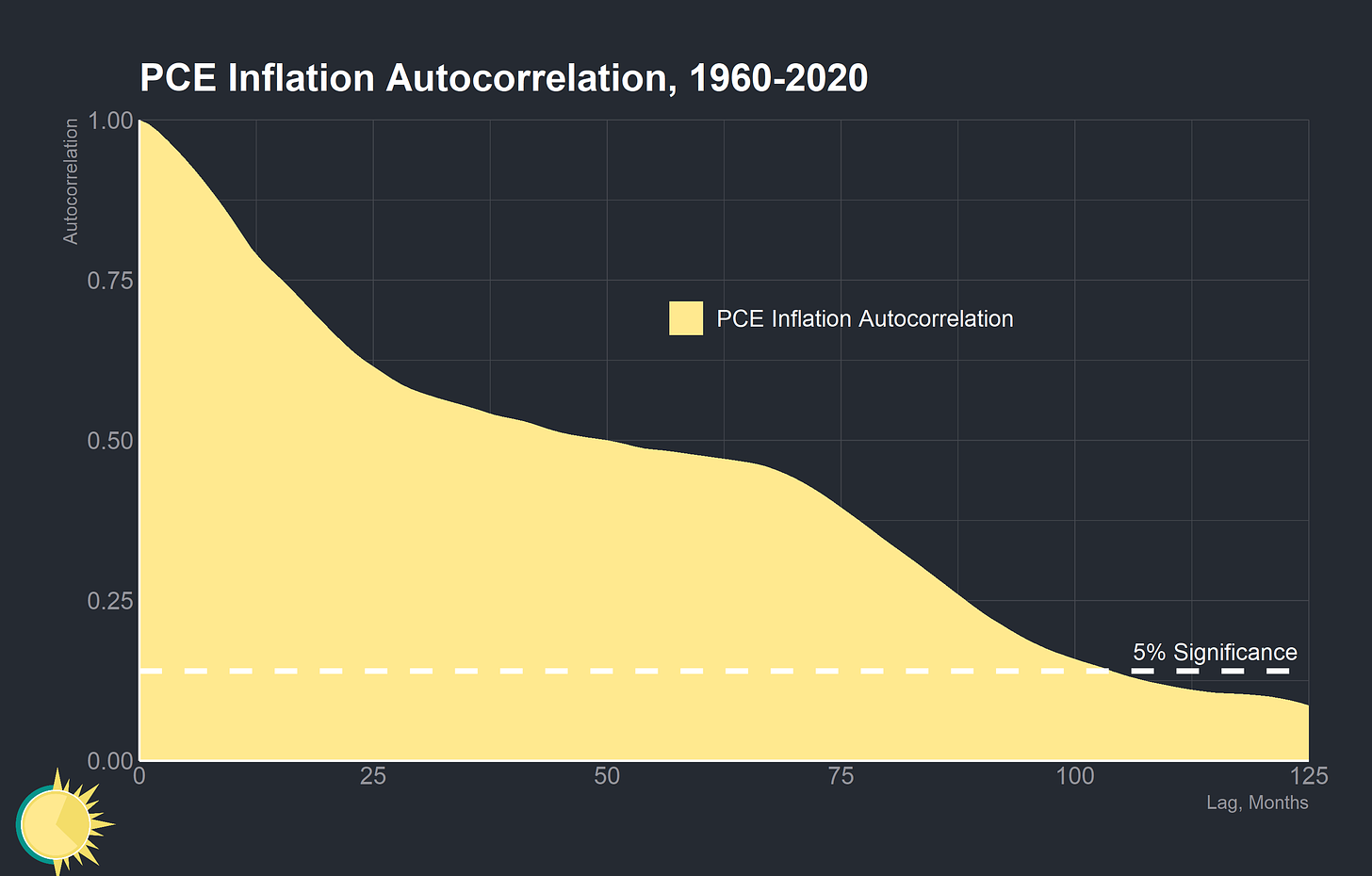
At a broader level, inflation is driven by more factors than just capacity utilization. Nominal income growth is primarily controlled by monetary policy, and high inflation can therefore occur separate from changes in labor utilization or capacity utilization. Supply shocks can also cause price shifts separate from nominal income growth. As shown in the graph above, inflation is also autocorrelated across periods as long as 9 years, meaning that high inflation in the past is correlated with high inflation now and the same is true with low inflation. Contracts based on nominal inflation expectations (like mortgages, union wage bargaining agreements, and so on) can make short term inflation expectations sticky through the political economy.

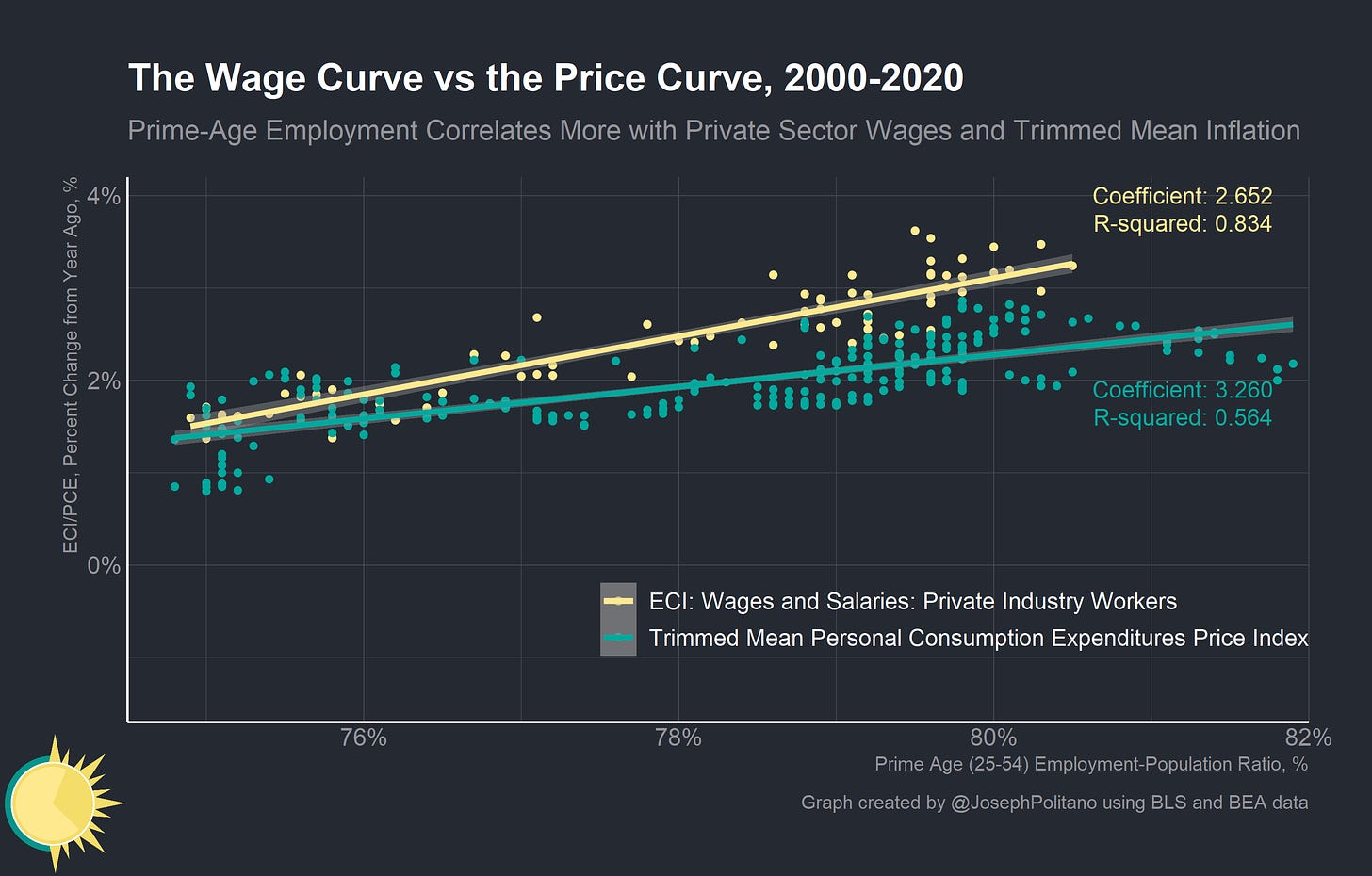
It is also important to acknowledge the relationship between labor utilization, wages, and prices. After all, A.W. Phillips’ original paper concerned itself with the relationship between nominal wage growth and unemployment—not inflation and unemployment. By using the prime-age (25-54) employment-population ratio, a better measure of employment that essentially calculates the percent of working age people who have a job, we can glean several insights about employment’s relationship with wages and prices.

As the graph above shows, higher prime age employment levels are generally correlated with higher nominal wage growth and nominal inflation as represented by the Employment Cost Index (ECI) and PCEPI respectively. Critically, the correlation is stronger and the slope is steeper for wage growth than it is for inflation. In short, this means that higher employment levels will generally produce higher real wage growth.

This relationship gets even stronger when using trimmed mean inflation, which cuts out the inflation components with the most fluctuations, and ECI wages and salaries for private industry workers.

However, it is important to acknowledge that the prime age employment Phillips curve is not particularly robust either. Though it does carry over to Japan, it does not hold up in either Canada or the United Kingdom.

The prime age employment Phillips curve holds up better than the traditional unemployment Phillips curve in Denmark, but still remains generally flat.

Fundamentally, it is worth acknowledging that no single variable or relationship will encompass the relevant theoretical macroeconomic tradeoff of the Phillips curve. There may be a theoretical short-term tradeoff between output and inflation, but it is not best expressed through unemployment and it is not consistently measurable in any one variable. Unobservable values like inflation expectations and potential output are critical in constructing the Phillips curve, and so attempts to conduct policy using it requires concocting unobservable values from tangential data and bad projections. All of this for a spurious, shifting, flat, and endogenous correlation.

Conclusions

At some level, it should be no wonder that the Phillips curve relationship does not survive intense scrutiny. All sorts of messy variables—inequality, expectations, random price fluctuations, public employment programs, price controls, aggregate policy responses—will affect the observed relationship. At a broader level, the seminal idea of the Lucas critique is that aggregate relationships in historical data cannot be used to accurately forecast policy effects or the economy writ large. Indeed, Lucas’s “Econometric Policy Evaluation: A Critique” was itself concerned in large part with reexamining the Phillips curve. Yet the Phillips curve persists in policymaking, discourse, education, and modelling.

Over the last two decades, America has fallen dramatically behind most of its G7 peer nations in terms of employment. There are several reasons for this—a dramatic housing shortage, a failure to provide basic childcare and parental leave, an inefficient healthcare system. But at the macroeconomic level, nothing has held us back more than the fear from policymakers at the Federal Reserve that unemployment would get “too low” and kick off inflation based on Phillips curve-style models.

It would be better if Federal Reserve policymakers were agnostic about the lower bounds of unemployment and focused their policy instead on generating stable nominal income growth. None of the G7 countries have had sustained bouts of inflation despite achieving higher employment levels than the US, so we should not worry about employment getting “too high.” In evaluating the labor market, policymakers should focus more on a combination of wage growth and employment levels and less on unemployment and its supposed natural rate. Only then will we be able to move beyond the confines of a Phillips curve framework and achieve full employment.

If you liked this post, consider subscribing to get free economics news and analysis delivered to your inbox every Saturday!